Cognitive Computing and Math for Increasing your Sales

Reading time: 20 minutes

In this post, I’d like to share some ideas, concepts, thoughts and a product I’ve been developing for several months in order to get some feedbacks, comments and thoughts from you.
I’ve been spending a lot time on thinking how to combine new technology trends (in particular cognitive computing, data science, big data, stream-based processing) and math in order to help businesses increase their sales. This is the holy grail of every business.
So, if my proposal resonates after sharing, please feel free to let me know your thoughts.

Every business should receive feedback from the customers in order to improve the processes and products and make the customers happier. Happy customers lead to more sales (with new sales, cross-selling and up-selling) and referrals to other potential customers.
At the end of the day, if you know what’s really important to your customers and you measure their experience (quality, service, environment, etc); then you can increase the customer’s engagement and finally increase your own sales.
A rule of thumb could be: “better feedbacks implies adapting your business and products that implies increasing customer’s loyalty that finally implies more sales“. One step further is getting and measuring feedbacks in real-time, so you can solve issues while the customer is still interacting with your business.

For example, hospitality and lodging industry is the one that lives and dies by the perception of customers and its own reputation by further comments. It’s well know that increasing the guests loyalty implies increasing the referrals and the ranking in social networks such as TripAdvisor and impacting positively on the revenue. So, it’s very important to hear and know what guests think about your business regardless if you’re the CEO, the revenue manager, the marketing manager or just the front-desk man.

So, we have key questions such as:

• How do I reach my customers in an easy and cost-effective way? Today, there are a lot of channels to reach the customers. Some are cheap (such as my web site, email, twitter, etc) while others are very expensive (TV ads, Super Bowl ads, etc).
• How do I reach my customer almost real-time in order to act pro-actively? I don’t want to wait several days for a phone interview. I’d like to know what’s thinking now or at least in the short-term.
• How do I gather and measure objectively what the customer thinks about? I need to use math and cognitive computing in order to measure objectively the customer’s experience by filtering out some subjectivity. As well, I need to make comparable different measurements/experiences in order to get correct insights.
• How do I influence my customers to send back feedbacks? For most of the customers, filling in old-fashion paper comment cards is not so good; so we need to design sexy and easy-to-understand comment cards to motivate the customers to fill it in.

The proposed solution is an information technology (for reducing cost and time to reach the customer) that displays an intuitive and sexy digital comment card (reducing paper costs and being eco-friendly) that helps to gather surveys easily and computes automatically the captured data (reducing computing time to get a result) and finally provides insights about your business for increasing the sales.

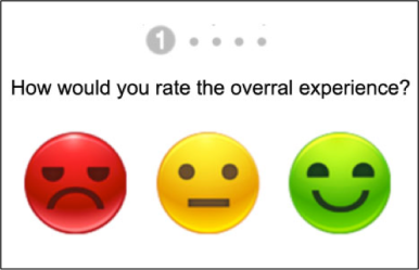
First of all, the product enables defining a questionnaire (a list of questions) for the digital comment card. When the digital comment card is sent to the customer, then five questions are randomly selected from the questionnaire and displayed to the customer in a sexy and easy-to-understand way as shown in the figure 01.

Figure 01

Then the customer select according to his/her experience. The product internally uses a math algorithm to convert the survey response into an actionable and objective index.
The idea is to assign a weight to each face and multiply by its distribution, so mathematically the index = sum(face_dist*face_weight).
Let’s suppose that we assign the weights as: bad_face_weight=0, neutral_face_weight =50 and happy_face_weight =100 and see some scenarios:

• If every response is bad, then we have the distribution bad_face_dist=100%, neutral_face_weight =0%, happy_face_weight =0% and the index is equal to 0*1 + 50*0 + 100*0 = 0 (the lowest index value)
• If every response is good, then we have the distribution bad_face_dist=0%, neutral_face_weight =0%, happy_face_weight =100% and the index is equal to 0*0 + 50*0 + 100*1 = 100 (the highest index value)
• If every response is neutral, then we have the distribution bad_face_dist=0%, neutral_face_weight =100%, happy_face_weight =0% and the index is equal to 0*0 + 50*1 + 100*0 = 50 (a medium index value)
• In the real world, we have a different distribution and index values between 0 and 100. Close to the 0 index is bad, close to the 100 index is good and around the 50 index is neutral

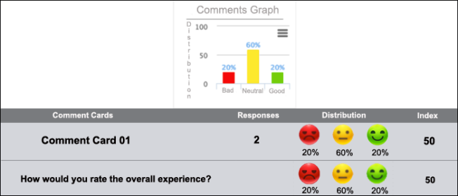
A key idea is to present a dashboard showing the number of responses related to the digital comment cards and the underlying index calculation. As well as, the product shows the calculated index for each question in the questionnaire. This is important to take actions correctly given the feedback per question and per whole comment card. You can see an example of dashboard in the figure 02.

Figure 02

It’s remarkable to say that the digital comment card may be accessed using different methods:

• A link embedded in an email, newsletter, Twitter message, Facebook post, etc
• Any device such as laptop, desktop, tablet, smartphone because it’s designed to be responsive (adaptable to any display device). By this method, you can locate a tablet in the front-desk, so the customer can respond the surveys while being in your business
• A QR code posted in your billboard, printed in a paper/newspaper/magazine or just send by any digital method

Finally, the product uses cognitive computing to discover insights from the customer comments. The product uses particular the technique named sentiment analysis part of the natural language processing discipline. It consists in analyzing a human-written text/comment and gives as a result the polarity of the text: positive (good for your business), negative (bad for your business) and neutral (neither good or bad) and set of concepts related to the comment.

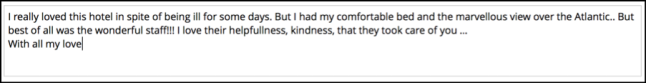
Let’s see a comment as shown in the figure 03.

Figure 03

We can discover several things in this comment as shown in the figure 04 such as the most important words related to the comment.

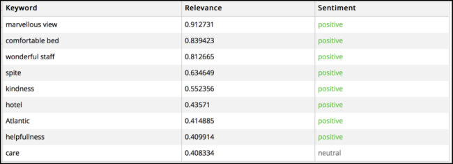
Figure 04

And the comment sentiment is shown in the figure 05.

Figure 05

The product enables to configure an email address for the case when we receive a negative comment in order to send an instant alert and act as fast as possible to solve any problem and improve the customer’s satisfaction.

I’m also thinking to include in the product the capability to discover customer segments using as an input the comments. I think to integrate the product with IBM Watson Personality Insight technology that extracts and analyzes a spectrum of personality attributes to discover the people personality. It’s based on the IBM supercomputer that famously beats humans at Jeopardy!.

Well, after sharing the key concepts and ideas of a product I’m developing, I’d like to hear from you if the problem/solution resonates to you, and if you’d like to participate in the beta testing phase.

You can reach at me: hello@nubisera.com and feel free to let me know your thoughts.

Juan Carlos Olamendy

CEO and Founder Nubisera

Nubisera Web Site

Reach Juan at juanc.olamendy@nubisera.com

A strategy for avoiding overfitting

By: Juan Carlos Olamendy Turruellas

When we build a predictive model, the key objective is the accuracy. Accuracy means that the model not only applies correctly to the training dataset but to the unseen dataset. When a model tends to predict/fit very good the training dataset (100% of accuracy) but tends to fail with unseen dataset (50% of accuracy), then it’s said that the model has overfit. Overfitting is a phenomenon that we need to deal with because all machine-learning algorithms have a tendency to overfit to some extent.

Researching on several books and Internet, I’ve discovered some patterns that allow me to formulate a strategy to avoid overfitting. I want to share this strategy for receiving feedbacks and improve it. In order to make it clear, I’ll materialize the concepts using some codes in Apache Spark and the spark-repl for running interactive commands.

The strategy can be visualized in the following roadmap in the figure 01.

Figure 01 

– Split randomly the dataset

The first step is to randomly split the original dataset into three non-overlapping datasets:

• Training dataset: to create predictive models
• Cross-validation dataset: to evaluate the parameters performance of the predictive models created using the training dataset
• Holdout dataset: to evaluate the performance of the best predictive models, and to measure how these models generalize correctly. These true values are hidden from the creation process of the predictive model and predicted values

We can see an example using Scala in Spark as shown in the figure 02.

Figure 02

– Build models

After that, we need to build predictive models using different values for the underlying parameters. In our example, we’re building a classifier using decision tree algorithms. We need to evaluate different options (for this kind of algorithm) for entropy, tree depth and bins (for more details, you can read the implementation in the Spark documentation). The output is a list of the tuple (model, precision, impurity, depth, bin).

The precision indicates how much the model is overfitting or generalizing by outputting a measure of true positive versus false positive. The higher value, the better accuracy.

It’s remarkable to say that these models are built using the training and cross-validation data set.

I illustrate the concepts using the following code as shown in the figure 03.

Figure 03

– Get top performance parameters

Next step is to see the parameters ordered by the best precisions as shown in the figure 04.

Figure 04

We can see for the case of decision trees the depth is what affects negatively on the predictive model accuracy. The less depth, the less accuracy.

Then, we get and print the top 5 performance parameters as shown below in the figure 05.

Figure 05

– Build and evaluate model with top performance parameters

Next step is to evaluate how accurate the best predictive models perform regarding to the hold-out/testing dataset. This step shows if the predictive models are really overfitting/memorizing the training data set or not.

We need to create a new training dataset comprising the former training and the cross-over datasets. We use the best parameters from the point of view to tune the model creation process.

The step is illustrated using the Figure 06.

Figure 06

– Print the best model

And finally, we can print how the best parameters perform with the hold-out dataset as shown in the Figure 07.

Figure 07 

It’s remarkable to say that these parameters build/create accurate models which don’t overfit. We can take any of these parameters to build the final predictive model which can be use accurately to predict unseen data points.

In this article, I’ve explained a strategy for avoiding overfitting in predictive models as well as the concepts are illustrated with real-world code in Scala/Apache Spark.

I look forward to hearing from you with your thoughts/comments/new ideas.

Installing a standalone Apache Spark cluster

In this post, I’d like to share my experiences about architecting and provisioning an Apache Spark cluster via scripts.

In these days, I’m working hard with customers for provisioning clusters and running machine learning algorithms in order to discover the most accurate predictive model on hundreds of billions of data rows. Because of the big amount of data rows, then the cluster tends to have several nodes; so we need to have some kind of scripts (in my case, for bash shell in Ubuntu 14.04) to automate and streamline (reduce working time) the creation of the cluster due to the number of nodes.

Conceptually, a standalone Apache Spark cluster is similar to other distributed architecture that I’ve designed for different technologies: Apache Mesos, load balancer+app/http_servers, MPICH, Hadoop file system/YARN, etc.

I mean we have a master node (sometimes a secondary node for service availability coordinated each other by ZooKeepers) and several worker nodes.

The master is the orchestra leader that coordinates the work to get done, deals with some possible failures and recovers, and finally gathers the results.

The worker nodes do the real hard work, data crunching and/or predictive model creation.

The communication channel between the nodes in the cluster is done using SSH.

A common deployment topology is like this:

• Master node:
  • Apache Spark viewpoint: We have the cluster manager that launches the driver programs (program with the data processing logic) and coordinates the computing resources for its execution. It’s like OS scheduler but at a cluster level
  • Hadoop FS viewpoint: We have the name node with the file system metadata. It contains the information of the tree structure and inodes and it knows where each data block resides physically in the cluster (in which data node)
• Worker nodes:
  • Apache Spark viewpoint: We have the executors. This is the runtime environment (computing resources container) where the tasks associated to the driver program logic are really executed. In this case, the tasks are executed in parallel (several tasks in the same node) and distributed (tasks on different nodes)
  • Hadoop FS viewpoint: We have the data nodes. This is where the data blocks (each files is divides in several data blocks) physically reside. Data blocks are distributed in the cluster for scalability/high performance and replicated by default at least in 3 nodes for availability (of course, we need at least 3 nodes in the cluster for this). Each data block is by default 64MB of size.

I can visualize the former deployment topology using the following diagram as shown in the figure 01.

Figure 01

These are the steps that I follow to create a cluster:

Step 01. In all the nodes, I configure the DNS (/etc/hosts) to associated hostname and IP correctly

Step02: In all the nodes, I create a user for running Spark and Hadoop under this security context. Let’s say sparkuser. As well as, I install the dependencies: Java and Scala

Step03. In the master node, I configure SSH login without password for root and sparkuser onto the worker nodes. For root user, it makes easy the automated provisioning. For the sparkuser user it’s required for running the Spark cluster. This is done using PKI mechanism and there are a lot of docs related

Step04. In all the nodes, I install and configure the base Hadoop as shown in the listing 01.

#!/bin/bash # Parameters for settings SPARKUSER=$(cat conf/spark.user.name.conf) SPARKMASTER=$(cat conf/spark.master.node.conf) HADOOPBASEDIR=$(cat conf/deploy.dir.conf) HADOOPCONF=$HADOOPBASEDIR/hadoop/etc/hadoop echo “—– Downloading and installing Hadoop 2.7.1 in the directory $HADOOPBASEDIR/hadoop” wget http://apache.mirrors.tds.net/hadoop/common/hadoop-2.7.1/hadoop-2.7.1.tar.gz tar zxvf hadoop-2.7.1.tar.gz rm -fr hadoop-2.7.1.tar.gz mv hadoop-2.7.1 $HADOOPBASEDIR mv $HADOOPBASEDIR/hadoop-2.7.1 $HADOOPBASEDIR/hadoop echo “—– Setting environment variables for Hadoop 2.7.1” echo -e “\n# Setting environment variables for Hadoop 2.7.1” >> /etc/profile echo “export HADOOP_HOME=$HADOOPBASEDIR/hadoop” >> /etc/profile echo ‘export PATH=$PATH:$HADOOP_HOME/bin:$HADOOP_HOME/sbin’ >> /etc/profile echo ‘export HADOOP_CONF_DIR=$HADOOP_HOME/etc/hadoop’ >> /etc/profile echo “—– Reloading environment variables for Hadoop 2.7.1” source /etc/profile echo “—– Configuring Hadoop 2.7.1” echo “—– Setting the hadoop-env.sh file” sed -i ‘s/${JAVA_HOME}/\/usr\/lib\/jvm\/java-8-oracle/g’ $HADOOPCONF/hadoop-env.sh echo “—– Setting the core-site.xml file” sed -i ‘s/<\/configuration>//g’ $HADOOPCONF/core-site.xml sed -i ‘$ d’ $HADOOPCONF/core-site.xml cat >> $HADOOPCONF/core-site.xml <<EOF <property> <name>fs.defaultFS</name> <value>hdfs://$SPARKMASTER:9000</value> </property> </configuration> EOF echo “—– Granting rights for the user $SPARKUSER on the Hadoop directory $HADOOPBASEDIR/hadoop” chown -R $SPARKUSER $HADOOPBASEDIR/hadoop

Listing 01

Step04a. In the master node, I configure the name node as shown below in the listing 02.

#!/bin/bash # Parameters for settings SPARKUSER=$(cat conf/spark.user.name.conf) SPARKMASTER=$(cat conf/spark.master.node.conf) HADOOPBASEDIR=$(cat conf/deploy.dir.conf) HADOOPCONF=$HADOOPBASEDIR/hadoop/etc/hadoop SPARKDATADIR=$HADOOPBASEDIR/hadoop/hadoop_data/hdfs/namenode #WORKERNODES echo “—– Configuring Hadoop platform on the master node $SPARKMASTER” echo “—– Creating directory” mkdir -p $SPARKDATADIR echo “—– Granting rights for the user $SPARKUSER on the Hadoop directory $HADOOPBASEDIR/hadoop” chown -R $SPARKUSER $HADOOPBASEDIR/hadoop echo “—– Setting the hdfs-site.xml file” sed -i ‘s/<\/configuration>//g’ $HADOOPCONF/hdfs-site.xml sed -i ‘$ d’ $HADOOPCONF/hdfs-site.xml cat >> $HADOOPCONF/hdfs-site.xml <<EOF <property> <name>dfs.replication</name> <value>3</value> </property> <property> <name>dfs.namenode.name.dir</name> <value>file://$SPARKDATADIR</value> </property> </configuration> EOF echo “—– Setting the masters nodes” echo “$SPARKMASTER” >> $HADOOPCONF/masters echo “—– Setting the slaves nodes” sed -i ‘$ d’ $HADOOPCONF/slaves for worker in $(cat conf/spark.worker.nodes.conf) do echo “$worker” >> $HADOOPCONF/slaves done

Listing 02

Step04b. In the worker nodes, I configure the data nodes pointing correctly to the name node as shown below in the listing 03.

#!/bin/bash # Parameters for settings SPARKUSER=$(cat conf/spark.user.name.conf) HADOOPBASEDIR=$(cat conf/deploy.dir.conf) HADOOPCONF=$HADOOPBASEDIR/hadoop/etc/hadoop SPARKDATADIR=$HADOOPBASEDIR/hadoop/hadoop_data/hdfs/datanode echo “—– Configuring Hadoop platform on the worker nodes” echo “—– Creating directory” mkdir -p $SPARKDATADIR echo “—– Granting rights for the user $SPARKUSER on the Hadoop directory $HADOOPBASEDIR/hadoop” chown -R $SPARKUSER $HADOOPBASEDIR/hadoop echo “—– Setting the hdfs-site.xml file” sed -i ‘s/<\/configuration>//g’ $HADOOPCONF/hdfs-site.xml sed -i ‘$ d’ $HADOOPCONF/hdfs-site.xml cat >> $HADOOPCONF/hdfs-site.xml <<EOF <property> <name>dfs.replication</name> <value>3</value> </property> <property> <name>dfs.datanode.data.dir</name> <value>file://$SPARKDATADIR</value> </property> </configuration> EOF

Listing 03

Step05. In all the nodes, I install and configure the base Spark as shown in the listing 04.

#!/bin/bash # Parameters for settings SPARKUSER=$(cat conf/spark.user.name.conf) SPARKMASTER=$(cat conf/spark.master.node.conf) SPARKBASEDIR=$(cat conf/deploy.dir.conf) echo “—– Downloading and installing Spark 1.4.1 in the directory $SPARKBASEDIR/spark” wget http://apache.mirrors.tds.net/spark/spark-1.4.1/spark-1.4.1-bin-hadoop2.4.tgz tar zxvf spark-* rm -fr spark-1.4.1-bin-hadoop2.4.tgz mv spark-* $SPARKBASEDIR mv $SPARKBASEDIR/spark-* $SPARKBASEDIR/spark echo “—– Setting environment variables for Spark 1.4.1” echo -e “\n# Setting Environment Variables for Spark 1.4.1” >> /etc/profile echo “export SPARK_HOME=$SPARKBASEDIR/spark” >> /etc/profile echo ‘export PATH=$PATH:$SPARK_HOME/bin:$SPARK_HOME/sbin’ >> /etc/profile echo “—– Reloading environment variables for Spark 1.4.1” source /etc/profile echo “—– Granting rights for the user $SPARKUSER on the Spark directory $SPARKBASEDIR/spark” chown -R $SPARKUSER $SPARKBASEDIR/spark echo “—– Configuring Spark 1.4.1 – File: spark-env.sh” cp $SPARKBASEDIR/spark/conf/spark-env.sh.template $SPARKBASEDIR/spark/conf/spark-env.sh cat <<EOF >>$SPARKBASEDIR/spark/conf/spark-env.sh export JAVA_HOME=/usr/lib/jvm/java-8-oracle export SPARK_PUBLIC_DNS=$SPARKMASTER export SPARK_WORKER_CORES=6 EOF

Listing 04

Step05a. And finally, in the master node, I do the configuration required to point to the worker nodes who will do the actual tasks/jobs as shown in the listing 05.

#!/bin/bash # Parameters for settings SPARKMASTER=$(cat conf/spark.master.node.conf) SPARKBASEDIR=$(cat conf/deploy.dir.conf) #WORKERNODES echo “—– Configuring Spark platform on the master node $SPARKMASTER” echo “—– Setting the slaves nodes” for worker in $(cat conf/spark.worker.nodes.conf) do echo “$worker” >> $SPARKBASEDIR/spark/conf/slaves done

Listing 05

Using the former scripts, I can automatically provision a standalone Apache Spark cluster with any number of worker nodes.

You can use it in your own provisioning and configuration, and I really appreciate if you let me know your thoughts/feedback/comments in order to improve it with your own scenario.

Collaborative Filtering in Apache Spark

One of the most important applications of machine learning in the business context is for the development of a recommender system. The most well known recommender engine is Amazon´s. There are two approaches to implement a recommender engine:

• Collaborative filtering: Base the predictions from user’s past behavior (rated, ranked or purchased items) in order to recommend additional items to users who made similar decisions. We don’t need to know the features (content) of the users or the items
• Content-based filtering: Base the predictions on the features of the items in order to recommend additional items with similar features

For our example, we’re going to use collaborative filtering approach because our dataset is in the format (user_id,item_id(movies),rating,timestamp) to recommend a list of movies to a user without knowing anything about the characteristics of the users and movies.

The driver for collaborative filtering comes from the assumption that people often get the best recommendations from someone with similar tastes and opinions to themselves. Apache Sparks implements Alternating Least Squares (ALS) algorithm as part of its MLLib library.

As the sample dataset, we’re going to use the movielens at http://grouplens.org/datasets/movielens/. The dataset summary is:

• data file contains the full dataset recording when a user rating a movie. Each row contains (user_id, movie(item)_id, rating, timestamp) separated by a tab
• user file contains the details of the users
• item file contains the details of the movies
• 100,000 rating (between 1 and 5)
• 943 users
• 1682 movies (items)

First step is to prepare the environment. Read the input file path from the environment variables and start a Spark Context as shown listing 01.

Listing 01

Next step is to represent the external data into an internal structure using a RDD and the case class Rating, by splitting each line by a tab separator and mapping fields to the case class Rating. Finally, we cache in memory the RDD because ALS algorithm is iterative and needs to access the data several times. Without caching, the RDD must repeatedly be recomputed each time ALS iterates. The code is shown in the listing 02.

Listing 02

Next step is to build the recommendation model.

It’s remarkable to say that there are two types of user preferences:

1. Explicit preference. Treats each entry in the user-item matrix as explicit preference given by the user to the item. For example, a rating given to items by users
2. Implicit preference. Getting an implicit feedback. For example, views, clicks, buy history

In this case, we’re using the ALS.train method as shown in the listing 03.

Listing 03

Next step is to evaluate the performance of the recommendation model as shown below in the Listing 04

Listing 04

Finally, if the performance is very good, we can start making recommendations for our users based on the former recommendation model. Let’s suppose that we want to make five movies recommendations for the user with id equal to 196, then we write the code as shown in the listing 05. Of course, to see the real name of the movies, we need to look for the u.item file by the returning values.

Listing 05

Now, we can apply this principles, knowledge and examples to your own solutions.

Computing statistics using Apache Spark

I’ve working heavily with the duet Apache Spark (for computing) and HDFS (as the distributed storage) for processing a very large volume of data. My customers want to get insights about their data and Apache Spark is a great tool for it. Using Apache Spark, I can crunch big data and compute statistics and generate predictive models using a bunch of machine learning libraries.

In this post, I want to show how simple is to compute statistics using Apache Spark and Scala.

The Apache Spark programming model is very simple. Our data is encapsulated in a RDD (Resilient Distributed Dataset). RDD is a monad that can be transformed by passing functions to its high-order functions (map, filter, foreach, countByValue, etc). Monads, functions and high-order functions are key concepts of functional programming and they’re well supported by Scala. It’s remarkable to say that RDD splits the data into partitions (data chunks) and distributes them onto the nodes of the cluster to process objects within a partition in sequence and multiple partitions in parallel. When we create a RDD, no execution takes place yet on the cluster; because RDD defines a graph of logical transformations over the dataset and the real execution takes place when we call an action (collect, foreach, counting, etc).

Let’s supposed that we have a big data file (aprox 1GB) with the following structure as shown in the listing 01. The last attribute (is_match) is a categorical one and the target. The remainder attributes are the features. We’re going to process the first (integer), second (integer) and the seven (optional double) ones.

“id”,”fea_1″,”fea_2″,”fea_3″,”fea_4″,”fea_5″,”fea_6″,”fea_7″,”fea_8″,”fea_9″,”fea_10″,”is_match” 37291,53113,1,?,1,1,?,1,1,1,0,TRUE 39086,47614,1,?,1,1,1.3,1,1,1,1,FALSE 70031,70237,1,?,1,1,?,1,1,1,1,TRUE 84795,97439,1,?,1,1,3.2,1,1,1,1,FALSE

Listing 01

Now let’s start writing code to process this data file. First of all, we need a representation of our data using a case class in Scala as shown in the listing 02. In this case, the data point has three features and its target. We also need a way to convert optional double to an internal representation using the toDouble function.

Listing 02

Next step is process the data file and get some statistics.

The very first step is to create a SparkContext object representing the communication with the cluster as shown in the listing 03.

Listing 03

Then we need to create a RDD from the SparkContext.textFile method to point the data file. Apache Spark can access to the local file system, distributed file system such as HDFS and Amazon S3 as well as databases such as Cassandra and HBase. When the RDD is created, then we can operate with transformations (transform the RDD into a new RDD) and actions (return a result to the driver program and trigger the real execution).

In our example, we filter out the header and for each line, split by the field separator and create instances of DataPoint case class. Finally, we persist the RDD in memory for reusing in the future. The code is shown in the listing 04.

Listing 04 

Next step is to create a histogram related to the target attribute (a categorical one). We’re going to use the countByValue method with a projection on the target property. This is an efficient implementation of the aggregation because when aggregating large dataset distributed in a cluster we’re facing with the network as the key bottleneck, so we need an efficient mechanism for moving the data over the network (serializing, sending over the wire and deserializing). The output is represented as Map[T, Long]. The code is shown in the listing 05.

Listing 05

If we want to get a histogram over a continuous variable, we need to use another way. We have to get a projection on the fea03 property. Then filter out the missing values and finally use the stats method as shown below in the listing 06.

Listing 06

In this post, I’ve shown how we can use Apache Spark for computing statistics for a very large dataset. You can apply this ideas and knowledge to your own scenarios.

Back to basics. Algorithm complexity

In these days, I’ve been thinking about basics courses when I was in the university studying computer science. There are some basics that IT professionals tend to forget because they think that the lessons learned are far away from everyday work. Paradoxically, there are a lot of lessons which are very closed to the reality with new IT challenges today. One of these forgotten but important lessons is algorithm complexity.

Today, when we (as software/solution/information architect and application designer) are normally faced with the need to crunch a big volume of data almost in real time using the most cost-effective way to make business decision right now.

The knowledge of algorithm complexity is mandatory in order to solve this kind of problems and make right decisions to impact positively in the application and the business. For example, if we have the ability to understand and choose the right data structure and algorithm; we can scale (growth without incrementing significantly the cost and effort) our software application without degradation when the volume of data or transactions increases; otherwise, we end up adding unnecessary computing resources.

Even today when computing resources tends to be cheap thanks to the cloud computing; from the business point of view it’s always necessary to reduce cost in order to save money and be more efficient and competent. In other words, it’s not the same to process a chunk of data with a cluster of 15 nodes than a cluster of 1000 nodes when we/our customers have to pay the bills.

Let me explain the principles around algorithm complexity and how it can help to save money to the business. The time complexity is used to represent how long an algorithm will take for a given amount of data. The mathematical expression to represent this notion is known as big O notation. What’s that? Well, big O notation is expressed by a mathematical function describing/providing as output how many operations an algorithm needs for a given amount of input data. Regarding to the mathematical function, the number of operations may/may not increase as the amount of input data increases.

The common used mathematical functions are:

• O(1). This is a constant complexity. It costs one operation no matter the amount of input data. For example, to lookup a data item in a hash table or to lookup a data item by its position in an array
• O(log(n)). The number of operations stays low even with a big volume of data. For example, to search a data item in a well-balanced binary tree when using a binary search
• O(n). The number of operations increases linearly as the amount of data increases. For example, to search a data item in an array
• O(log(n)*n). The number operations increase significantly as the amount of data increases. For example, sorting data items using efficient sorting algorithms such as QuickSort, HeapSort and MergeSort
• O(n²). The number of operations explodes quickly as the amount of data increases
• O(n³), O(2ⁿ), O(n!), O(nⁿ). There are a lot of worst complexities when the number of operations explodes significantly. These are bad time complexities. You should never design an algorithm with a complexity above O(n!) otherwise you should ask yourself if designing and implementing applications is really your field

We can visualize the complexity of different functions (amount of input data à number of operations) as shown below.

Now let’s see the concepts with concrete examples.

For example, when the amount of data is low, there is no significant different between O(1) and O(n²) algorithms on data processing because the current processors can handle hundreds of billions of operations per second.

Let’s suppose that we want to process 10,000 data items, we have the following scenario:

• O(1). It costs 1 operation
• O(log(n)). It costs 13 operations
• O(n). It costs 10,000 operations
• O(log(n)*n). It costs around 130,000 operations
• O(n²). It costs 10,000,000,000

As we can see the O(n²) algorithm costs 10,000,000,000 operations which may occur in a fraction of a second with the current processors.

Now let’s supposed that we want to process 10,000,000 data items. It’s really not a big database today. We have the following scenario:

• O(1). It costs 1 operation
• O(log(n)). It costs 23 operations
• O(n). It costs 10,000,000 operations
• O(log(n)*n). It costs around 230,000,000 operations
• O(n²). It costs 100,000,000,000,000 operations

As we can see the O(n²) algorithm costs 100,000,000,000,000 operations. We can go to take a long sleep while the processing is done.

Now we can see why we, as architect and application designer, must understand deeply the problems and select the right data structure and algorithm for the underlying solutions. If we select the right algorithm/data structure with a low complexity, we’re choosing the way to appropriately scale the application, in other words, to add the right computing resources when the volume of data and/or transactions increases impacting positively on saving a lot of money to our customers.

Getting the most frequently words in a text

In the recent days, I’ve been involved in the design of high performance and scalable architectures for data science solutions.

So, I would like to share some interesting insights, cookbook recipes and best practices that I’ve discovered and embraced.

In this post, I want to show you how to get the most frequently words in a text using simple data science techniques.

First of all, I want to say that sometimes when I design a data science solution and of course it’s up to the particular scenario, I try to express and validate the proposed algorithm using Unix commands connected by a pipeline before implementing the final logic in distributed platform such as Apache Spark. At the end of the day, this is the fastest way to express and tune the business logic before going to a solution more scalable.

The common use case related to this particular problem is to get a knowledge about the real main theme and thought process of a person delivering a text/speech/book to an audience. For example, when politicians deliver a speech, we can see what’s really the purpose of his own words by reading between the lines, getting insights and leaving out what’s not important.

In this post, we’re going to examine the book “The Adventures of Sherlock Holmes” extracted from the Project Gutenberg.

The solution logic is express in the following steps:

1. Scan the text and produce a list of lines
2. For each line, we extract the words, and produce a list of words
3. For each word, we standardize by converting each word to lower case
4. We group the word, and count them
5. We sort the words by frequency (the most frequent in the top)
6. And finally, we print the 10 most frequently words

The Unix command version is express as shown in the listing 01.

> cat pg1661.txt | \ #Step01 > grep -oE '\w+' | \ #Step02 > tr '[:upper:]' '[:lower:]' | \ #Step03 > sort | uniq -c | \ #Step04 > sort -nr | \ #Step05 > head -n 10 #Step06 Listing 01

Now we need to translate this logic into Apache Spark platform using Scala language as shown below in the listing 02.

import org.apache.spark.SparkContext import org.apache.spark.SparkContext._ import org.apache.spark.SparkConf object App { val Input_Datafile_VarName = "INPUT_DATAFILE" def getEnvVar(name: String): Option[String] = Option(System.getenv(name)) def processDataFile(input: String) { val conf = new SparkConf().setAppName("App") val sc = new SparkContext(conf) println("Reading the data file %s in memory cache".format(input)) val ds = sc.textFile(input).cache() //Step01 val result = ds.flatMap(x => x.split("\\W+")).filter(!_.isEmpty) //Step02 .map(_.toLowerCase) //Step03 .map(w=>(w,1)).reduceByKey(_+_) //Step04 .sortBy(_._2,false) //Step05 .take(10) //Step06 result.foreach(println) } def main(args: Array[String]) { val inputFile = getEnvVar(Input_Datafile_VarName) for { input <- inputFile } processDataFile(input) println("Ending the Spark application") } } Listing 02

After building the package, we can run it using the following commands as shown below in listing 03.

> export INPUT_DATAFILE=pg1661.txt > spark-submit --class "App" --master local[2] target/scala-2.11/my-project-assembly-1.0.jar Listing 03

Conclusion

Now we can use this solution in your own data science toolbox.

A tutorial on Node.js for dummies

 

In this world of high performance (low response time on almost real-time communication) and scalable (involving millions of user requests) Web applications, Node.js is gaining popularity everyday. Some says that Node.js is the hottest technology at Silicon Valley used by tech giants such as VMWare, Microsoft, LinkedIn, eBay, Yahoo, etc.

Let’s say what is Node.js?

In simple words, Node.js is an event-driven JavaScript runtime environment on the server-side. Node.js runs using V8 JavaScript engine developed by Google and achieves high throughput via non-blocking (asynchronous) I/O in a single-threaded event loop as well as due to the fact that V8 compiles JavaScript code at high speeds into native machine code.

The real magic behind the high performance on Node.js is the event loop. In order to scale to large volumes of user requests, all I/O intensive operations are performed asynchronously. The traditional threaded approach where for processing each user request a new thread is created is cumbersome and consumes large unnecessary resources specifically memory. To avoid this inefficiency and simplify the traditional multi-threaded programming approach, then Node.js maintains an event loop which manages all asynchronous operations for you. When a Node.js application needs to execute an intensive operations (I/O operations, heavy computation), then an asynchronous task is sent to the event loop along with a callback function, and then keep on executing the rest of the application. Then the event loop keeps track the execution status of the asynchronous task, and when it completes the callback is executed/called by returning results to the application.

The event loop efficiently manages a thread pool and optimized the execution of tasks. Leaving this responsibility to the event loop, allows the developers to focus on the application logic for solving the real problem and finally simplifying the asynchronous programming.

Now, let’s go to the practical part of this article. We’re going to install Node.js, and create a MVC framework for starting to develop our Web application.

In order to install Node.js, we need to follow the simple instruction in the official site at https://github.com/joyent/node/wiki/Installation.

Our MVC framework comprises of the following architectural building blocks:

• a HTTP server for serving HTTP requests. Unlike other development stack where the application server (ex, Tomcat) and web server (ex, Apache) are distinct modules in the solution architecture, in Node.js  not only we implement the application but also we implement the HTTP server
• a router in order to map HTTP requests to request handlers. This mapping is based on the URL of the request
• a set of request handlers to fulfill/process the HTTP requests arrived to the server
• a set of view to present data/forms to the end user
• a request data binding mechanism in order to understand correctly the data carried onthe incoming HTTP request payload

It’s remarkable to say that we’re going to implement each building block on its underlying module in order to follow/comply the very architectural principles: separation of responsibilities to achieve loosely coupling and high cohesion.

The HTTP server

In this section, we’re going to implement the HTTP server building block of our architecture. Let’s create the server.js module in the root directory of the framework with the following code in Listing 01.

var http = require(“http”); function start() {    http.createServer(       function(request, response) {          console.log(“HTTP request has arrived”);          response.writeHead(200, {“Content-Type”: “text/plain”});          response.write(“Hello World”);          response.end();    }).listen(8888);   console.log(“Server has started at http://localhost:8888/“); } exports.start = start;

Listing 01. Module server.js

Let’s analyze the previous code. The first line requires the http module that ships with Node.js and make it accessible through the variable http. This module exposes the createServer function which returns an object, and this object has method listen which receives as input parameter the port is going to listen on. The createServer function receives as input parameter an anonymous function with the logic of the Node.js application. This anonymous function receives as input parameters a request and response objects used to handle the details in the communication with client-side. In this case, we don’t use the request object as well as the response.writeHead sets the HTTP status 200 (OK) and the content type, the response.write sends the content/data to the client-side and finally the response.end closes the communication. Whenever a HTTP request arrived at Node.js, the anonymous function is called (technically, this anonymous function is a callback handler to the on_request events). In this case, whenever a new request arrives, then the message “HTTP request has arrived” is printed on the command line. You may see this message twice, because most modern browsers will try to load the favicon by requesting in this case the following URL http://localhost:8888/favicon.ico.

Finally, the server bootstrapping logic is encapsulated in the start function which is in turned exported by the server.js module.

In next step, let’s create the main module index.js which is used to connect and initialize the remaining modules as shown in the Listing 02. In this case, we’re going to import the server.js internal module and call the start function.

var httpServer = require(“./server”); httpServer.start();

Listing 02. Module index.js

And finally, let’s run this first part of the application in your terminal as shown in Listing 03.

node index.js

Listing 03

The router and request handlers

Now, we can process a HTTP request and send a response back to the client-side. But, the common in Web application is to do something different depending on the URL associated to the HTTP request. So, we need another abstraction called the router which main feature is to decide which logic to execute based on URL patterns.

Let’s suppose that we’re developing a Web application with three features exposed as /app/feature01, /app/feature02 and /app/feature03.

First of all, let’s create the requestHandlers.js module with the handlers definition as show in the following listing. The handler definition is very simple: we’re just returning a string to display on the browser. If you want to parse the query string or bind the posted form data, the querystring module must be used.

function feature01(request, response) {         console.log(“HTTP request at /app/feature01 has arrived”);         response.writeHead(200, {“Content-Type”: “text/plain”});     response.write(“Feature01 is called”);     response.end(); } function feature02(request, response) {         console.log(“HTTP request at /app/feature02 has arrived”);         response.writeHead(200, {“Content-Type”: “text/plain”});     response.write(“Feature02 is called”);     response.end(); } function feature03(request, response) {         console.log(“HTTP request at /app/feature03 has arrived”);         response.writeHead(200, {“Content-Type”: “text/plain”});     response.write(“Feature03 is called”);     response.end(); } exports.feature01 = feature01; exports.feature02 = feature02; exports.feature03 = feature03;

Listing 04. requestHandlers.js module

Then, let’s create the router.js module with the definition of routing logic as shown in the following listing. In this case, the router receives as input parameters the list of handlers in dictionary form (name == url pattern and value == reference to the underlying request handler), the pathname representing the current url, request and response objects.

function route(handlers, pathname, request, response) {     if (typeof handlers[pathname] === ‘function’) {          handlers[pathname](request, response);     } else {         response.writeHead(400, {“Content-Type”: “text/plain”});         response.write(“404 Resource not found”);         response.end();     } } exports.route = route;

Listing 05. router.js module

Next, we need to refactor the server.js module as shown in the following listing. The url module is required to extract the part of the URL.

var http = require(“http”); var url = require(“url”); function start(route, handlers) {    http.createServer(       function(request, response) {          console.log(“HTTP request has arrived”);                   var pathname = url.parse(request.url).pathname;          route(handlers,pathname, request, response);    }).listen(8888);   console.log(“Server has started at http://localhost:8888/“); } exports.start = start;

Listing 06. Refactoring of server.js module

And finally, let’s refactor the index.js module to register the application URLs and wire the framework modules as shown in the following listing.

var httpServer = require(“./server”); var requestHandlers = require(“./requestHandlers”); var router = require(“./router”); var handlers = {} handlers[“/app/feature01”] = requestHandlers.feature01; handlers[“/app/feature02”] = requestHandlers.feature02; handlers[“/app/feature03”] = requestHandlers.feature03; httpServer.start(router.route, handlers);

Listing 07. Refactoring module index.js

Now let’s refactor our application to present a Web form and process the input data. Let’s suppose the /app/feature01 is Web form and the /app/feature02 is the endpoint for form processing.

Now let’s create the views.js module with the definition of the Web form related to the /app/feature01 as shown in the following listing.

function feature01View() {  var html = ‘<html>’+             ‘<head>’+             ‘<meta http-equiv=”Content-Type” content=”text/html; charset=UTF-8″ />’+             ‘</head>’+             ‘<body>’+             ‘<form action=”/app/feature02″ method=”post”>’+             ‘<input type=”text” name=”data” id=”name”></input>’+             ‘<input type=”submit” value=”Submit data” />’+             ‘</form>’+             ‘</body>’+             ‘</html>’;   return html; } exports.feature01View = feature01View;

Listing 08. views.js module

Next, we need to refactor the feature01 request handler to send back to the end user the Web form as shown in the following listing.

var views = require(“./views”); function feature01(request, response) {         console.log(“HTTP request at /app/feature01 has arrived”);         response.writeHead(200, {“Content-Type”: “text/html”});     var html = views.feature01View();     response.write(html);     response.end(); }

Listing 09. Refactoring the feature01 request handler function

Now, we have a very interesting way to process POST HTTP request. Because in Node.js the key concept is to process anything in an asynchronous way, then Node.js delivers to our application code the posted data in chunks through callbacks to specific events on Node.js. The data event is called when a new data chunk is ready to be delivered to the application code while the end event is called when all the data chunks are received by Node.js and ready to be delivered to the application code.

Now, we need to refactor the server.js module in order to add logic to select how to process GET or POST methods as shown in the following listing. In the case of the GET method, everything is same as before (no changes). In the case of POST method, we do the following steps:

1. define that the expected data is encoded using utf8
2. register a listener callback for the event data to be invoked every time a new chunk of posted data arrives, and then we append every chunk to the resultPostedData variable
3. register a listener callback for the event end to be invoked when all the posted data is received and ready to be delivered to the underlying request handler passing the  resultPostedData as parameter

var http = require(“http”); var url = require(“url”); function start(route, handlers) {    http.createServer(       function(request, response) {          console.log(“HTTP request has arrived”);          var resultPostedData = “”;          var pathname = url.parse(request.url).pathname;          if(request.method==’GET’)          {            route(handlers,pathname, request, response);          }          else          if(request.method==’POST’)          {            request.setEncoding(“utf8”);            request.addListener(“data”, function(chunk) {                resultPostedData += chunk;            });            request.addListener(“end”, function() {                route(handlers, pathname, request, response, resultPostedData);            });          }    }).listen(8888);   console.log(“Server has started at http://localhost:8888/”); } exports.start = start;

Listing 10. Refactoring of server.js module

We also need to refactor the router.js module as shown in the following listing.

function route(handlers, pathname, request, response, postedData) {     if (typeof handlers[pathname] === ‘function’) {          if(postedData === undefined)         {            handlers[pathname](request, response);         }         else         {             handlers[pathname](request, response, postedData);         }     } else {         response.writeHead(400, {“Content-Type”: “text/plain”});         response.write(“404 Resource not found”);         response.end();     } } exports.route = route;

Listing 11. Refactoring of the router.js module

And finally, let’s refactor the feature02 request hander as show in the following listing.

function feature02(request, response, postedData) {         console.log(“HTTP request at /app/feature01 has arrived”);         response.writeHead(200, {“Content-Type”: “text/html”});     response.write(“Posted data is”+postedData);     response.end(); }

Listing 12. Refactoring the feature02 request handler function

And to finish this tutorial, I will explain how to return JSON formatted objects to the client-side. This is  one the brightest features of Node.js because we can build a very scalable and fast back-end on Node.js and later to consume the related services from any client-side technology that understand simple HTTP such as browser, mobile application, etc.

Because we have developed a good framework, then we only need to refactor the feature03 as shown in the following listing.

function feature03(request, response, postedData) {         console.log(“HTTP request at /app/feature01 has arrived”);         response.writeHead(200, {“Content-Type”: “application/json”});     var anObject = { prop01:”value01″, prop02:”value02″}     response.write(JSON.stringify(anObject));     response.end(); }

Listing 12. Refactoring the feature02 request handler function

I hope this tutorial on Node.js for dummies is very helpful for you.

I look forward to hearing from you comments anytime you like …

Lessons Learned: What could be a great business idea

 

I spend part of my time thinking how to provide solutions using IT technologies. I would like to share some insights that I´ve concluded on my short career as entrepreneur. In this article, I´m talking about what could be a great business idea.

If you want to make this world a better place providing your own technological solutions and decide to run your own business (aka becoming an entrepreneur); from my humble point of view there are some elements that contribute to the success of a business idea and they´re highly considered by investor when evaluating your proposal.

If you can apply math and create a formula by factoring the key elements on evaluating the potential of a business idea; it should be similar to:

Sucessful business idea = big market + unfair advantage (defensible product) + very good traction + scalable business model

Let´s talk about these factors a little bit more.

• Big market: A big market offers the potential of monetize at a large scale as well as it gives you the room to pivot the business model onto different directions without changing the target market. You can discover big market by doing market research and reading the trends on the IT market on the reports from IDC, Gartner, Yankee Group, etc
• Unfair advantage (defensible product): Defensibility is essential to survive in today highly competitive global markets; specially when you face large companies with unlimited resources that could act as copy-cats. There is no right strategy or silver bullet for this aspect and it´s up to your creativity
• Very good traction: If you have a good traction, then your product is making happy your customer by solving a real pain (problem). Your customers are using product so frequently, so the churn rate is low which is equal to that the customer lifecycle is expanded in the time; and therefore your stream of revenue increases positively. As well as, if your product is sticky (again, equal to happy customers), then your customers can speak very well about your product (impacting positively on the word-of-mouth marketing channel — your own customers can/could become part of your sales force indirectly), then producing the disired viral effect on the product; therefore increasing your customer base and more importantly reducing your cost of customer acquisition.
• Scalable business model: This is the interception between revenue streams and cost structure, or how you make money. If you achieve a scalable business model by acquiring customers (CAC) very less costly than the profit of the entire lifecycle of your customer (CLTV) using your product (CLTV>3CAC) and you achieve a very low marginal cost (cost of providing another unit of service related to your product); then you are doing very good and ready to scale (it´s not costly to grow) your business model to its maximum potential (the machine makes more money)

Although there could be a lot of factors to evaluate what could be a great business idea; I consider the aforementioned the essentials to discovery a successful business model and run your own company.

I would really appreciate to hear different worldviews, so what do you think about?

The simplest way for archiving and searching emails

In this article/post, I want to share with the entrepreneur community a new business idea that I have in mind in order to get feedbacks, comments and thoughts (I would really appreciate it). As a software and enterprise architect, I´m always designing simple, usable (functional) and pretty (good user experience from the aesthetic view) architecture solutions and refactoring to optimize the architecture of legacies. I´m a fond of optimization problems (research and practice), specifically in the topics of high performance for storage, indexing and processing. Applying the customer development and lean startup concepts, my vision is to (re-)segment the problem/solution space of data archiving toward the email archiving. So, I´m thinking to make my contribution to the computer world by providing an optimized email archiving solution in terms of storage cost effectiveness and simple user interface for organizing and searching emails very easily (this is my unique value proposition). I´m guessing that the target market (customer segment in the business model canvas) are personal-, small-, and medium- business which mainly need to store/archive the emails for legal and particular purposes in a large period of time. I want to name this service as Archivrfy.

Business transactions not only can involve enterprise applications and OLTP systems but also a bunch of emails, for example to register contracts, sales conversations and agreements as well as for evidence of invoices and payment information. Most companies underestimate the effort for the maintanance of traditional tape backups and data indexing to simplify searches.

In order to protect and retain mission critical data contained in emails; companies need a new and very simple approach to easily capture, preserve, search and access emails. For example, the legal department and people see e-mail as an essential factor in its discovery response strategy to present them as evidence in a court of law. The volume of email being generated every day is becoming a huge problem, so organizations and people can free its storage space by moving emails to archiving vaults.

You can archive emails at low cost for reducing local storage space and complying with legal requirements. For security, data is encrypted while in transit and preserve in the final vaults using adjustable retention policy. It´s based on cloud computing technology and available always with 99.99%. It´s scalable with unlimited growth (depending on the available resources in the cloud).

You can use a very simple and fast user experience to search (supporting eDiscovery scenarios) and access to the archived emails for improving productivity. It´s based on an optimized search algorithm by enriching the content with metadata to organizing and extending dynamically the search criteria. As well as it´s a flexible tecnology for simple integration with existing platforms and exporting to several portable email files.

In order to support the previous scenearios using a solution with scalability, high availability and high performance in mind; we need to design a robust architecture for Archivrfy service as shown below.

In this article, I´ve share my vision of an email archiving solution in terms of the unique value proposition and the underlying technical architecture.

I really appreciate any thoughts and feedback to help me improve my business vision.

I look forward to hearing from you … very soon